Author: safety
-

trippler – and resilience for all
After driving an EV at possibly the busiest Australian road-tripping time of the year (Easter), in the middle of a global fossil fuel crisis and concomitant surge in local EV sales, I decided it was time to make good on my claim that resilient planning by individuals could benefit all drivers. In practice, this means…
-

Antifragile AI Architectures
AI is full of contradictions: capable but unreliable, local improvements create externalities, generalist models are evaluated against specific criteria, and so on. Antifragility is a framework that deals in contradictions too, and seems an appropriate lens through which to explore AI systems architecture, as I had used it in an earlier era to explore hand-crafted…
-

Data and AI mini blogs
A brief reflection on Thoughtworks Australia Data & AI mini-blogs. From May 2021, we set ourselves a target to publish a short blog on a different AI, ML or data topic every week. Here’s the pitch from the landing page: Bite-sized content delivering valuable insights from Thoughtworkers who wrestle varied client problems week in and…
-

LLMs are lineage black holes
Data lineage is important to most organisations, even if they don’t make use of it. Systematically capturing the upstream provenance and downstream consumers of any piece of data is critical to trusting the utility of that data and understanding its impacts, at any scale beyond a handful of excel spreadsheets. The nature of lineage When…
-

LLMs as text simulators
I’ve often written here about developing systems that leverage simulation. Simulation combining physical processes, information systems, and crowd behaviours. Simulations that support organisational decision making, customer experiences, and learning. And in late 2025 we were having a moment where more people were starting to describe Large Language Models (LLMs) as simulators of text. Simulation of…
-

trippler at Melbourne Python meetup
I recently presented a version of my PyConAU trippler talk at the February 2026 Melbourne Python meetup. I made a few minor updates, such as incorporating the new contingency and multi-destination functionality, and this may have caused me to run a little over time… Running a little over time must have angered whatever deities watch…
-

Ignore all previous instructions – Snow Crash cosplay
With an end-of-year party themed Enter the Simulation, I had to cosplay Snow Crash, the book that coined the term “metaverse”. Spolier alert: Skip ahead to the build notes, or read on for the explanation, which Neal Stephenson fans and tech nerds may have already pieced together… The eponymous Snow Crash virus from the 1992…
-
trippler multi-destination
It’s time for my EV trip planning app trippler to cater to multiple destinations, beyond the beaten track of simple A-to-B trips. This is another feature I decided I needed when planning and driving The Cross to The Cape. Multiple changes I’ve wanted multiple destinations for some time, but recent refactoring of the UI and…
-
trippler contingencies
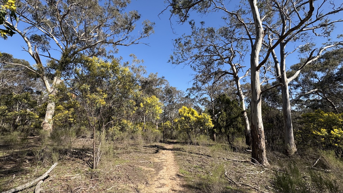
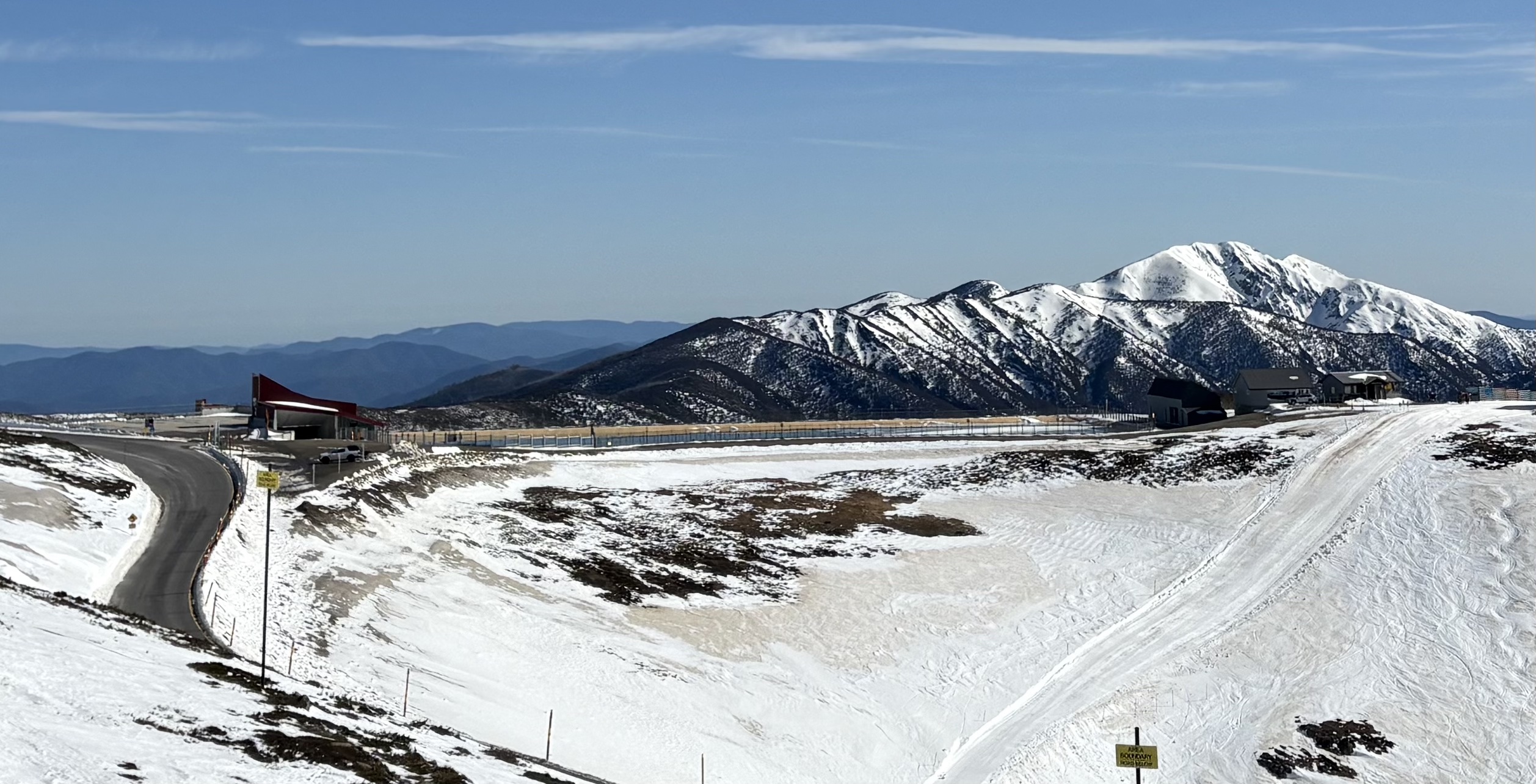
Planning a dawn-to-dusk adventure from snow to surf in an electric vehicle meant not just planning for resilience, to allow for changes to the plan, but also planning for contingencies, to know in advance exactly how to respond to changes. Carnival of carving We lay our scene on the descent from Mount Hotham to Cape…
-
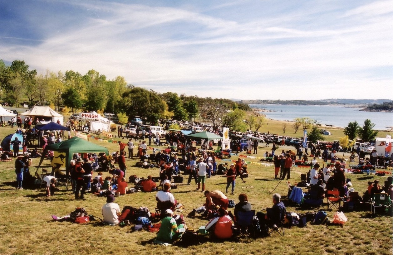
Orienteering map training turns 20
A little over 20 years ago, I was introducing my wife and some friends to orienteering in Jindabyne. With my family involved in the Scottish 6 Days since its 1977 inception, I had been orienteering since before I could walk, and reading orienteering maps was second nature to me. Not second nature to the rest…