Category: Machine Learning
-

22 rules of generative AI, 2 years on, part 1
How has my original post on 22 rules of generative AI aged in a period of rapid change? Are these solution considerations as enduring as I thought? Let’s reflect on the original advice and developments in the meantime. Apologies again for minimal references as I timeboxed the writing. In general, evidence should be discoverable/verifiable with…
-

AI conversations for every role
We always envisaged Effective Machine Learning Teams (EMLT) speaking to multiple roles. Recently we’ve spoken to 4 distinct audiences about ML development, and you can listen in too. Whether you identify with: there’s a podcast* for you with popular presenters – see more below. Product We joined a Product Tank Melbourne event, along with Ana…
-

Joe Reis show
I had a great chat with Joe Reis on The Joe Reis Show, along with one co-author of Effective Machine Learning Teams, David Tan. We covered the motivation for the book, scenarios where we’d helped teams address issues to become more effective, and the tools we’d developed from those solutions. We also talked about a…
-

Effective topologies for Data and ML teams
I presented this talk at the Melbourne Data Engineering meetup, on a wild and wet Friday night. Having your cake and eating it too – Effective topologies for Data and ML teams (slides) In the talk I explore how Team Topologies provides patterns for reconciling fast flow of value with (multiple) specialisations in data and…
-

GenAI stone soup
GenAI (typically as an LLM) is pretty amazing, and you can use it to help with tasks or rapidly build all kinds of things that previously weren’t feasible. Things that work some of the time. The soup But do you find yourself reworking large chunks of generated content, or face major hurdles in getting a…
-

Hopsworks and multidisciplinary ML
I recently had a brief but fun chat with Hopsworks about the multidisciplinary nature of building machine learning products, as part of their 5-minute podcast series hosted by Rik Van Bruggen. See the transcript and video at 5-minute-interview-with-david-colls-nextdata. Rik and I talked about how David, Ada and I address this multidisciplinary perspective in our book…
-

Demistifying ML product teams
Along with Ana Kelk, Head of Product (ecosystem) at Canva, David Tan, Ada Leung and I participated in a panel for Product Tank Melbourne, discussing the particular needs of ML product development (and the common product development needs too!) It was a great way to share and get feedback on one of the key themes…
-
Effective ML Teams on Thoughtworks Tech Podcast
I recently recorded an episode of the Thoughtworks Technology Podcast with my Effective Machine Learning Teams co-authors Ada Leung and David Tan, hosted by Scott Shaw and Ken Mugrage. The episode is number 146 – Building at the intersection of machine learning and software engineering. It was great to chat about the book and share…
-

EMLT Q&A
A fun Q&A with Thoughtworks on the drivers, key messages and writing process for Effective Machine Learning Teams (EMLT) with my fellow authors Ada and David. It’s neat to be featured alongside all the other many great books from Thoughtworks authors. Find the book, trial and purchase options at O’Reilly, and find yourself a nice…
-
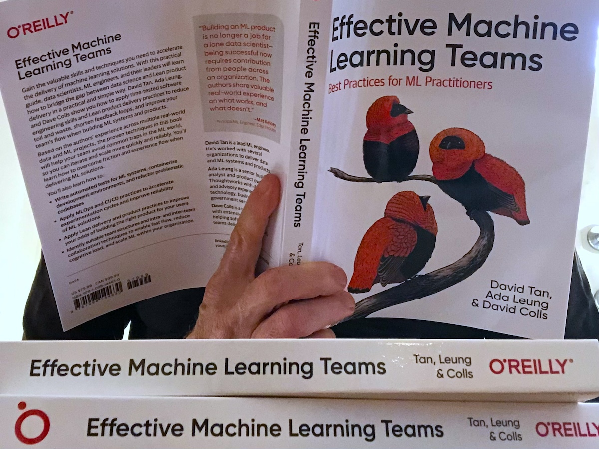
Effective Machine Learning Teams in print
My book Effective Machine Learning Teams is now in print! Building ML solutions requires multi-disciplinary collaboration. EMLT shows how to use design practices to identify the right products, how to apply good data science and software engineering practices to build products right, and how to structure ML teams and organisations so that they are right…