Sure commercial maps app directions are great, but have you ever found the customisation options limited? What if you want to use bike paths and back streets when cycling, or avoid winding roads that might make backseat passengers car-sick on a road trip?

The paved route
OpenStreetMap and OpenRouteService do provide this type of functionality, and could be considered for use as-is or with further customisation. PostGIS and pgRouting provide capabilities if you bring your own data. Many dedicated apps support groups with particular mobility needs.
My way, off the highway
In researching these capabilities however, and because I’m a fan of maps and I wanted to understand the whole data transformation journey, I decided to hand-roll my own navigation solution using pyshp, numpy, scipy, and networkx, all visualised with matplotlib. The end result is far from polished, but it can ingest 1.1M road geometries for the Australian state of Victoria, and generate a topological graph for routing within minutes, then use that map to to generate turn-by-turn directions in real time.
See the source code and the brief write-up below if you’re interested.
Data
The solution uses data from the Vicmap Transport data set, which provides road centrelines for highways, streets, tracks, paths, etc, for all of Victoria and some bordering regions. The spatial features are augmented with 71 attributes useful for routing, including road names, permitted directions of travel, height limits, etc. I used a GDA2020 datum grid projection shapefile export. Pyshp provides a list of geometries and attributes via shapeRecords.
Topology
Vicmap Transport road centrelines are collections of polylines. The endpoints of these polylines (aka road segments) helpfully coincide where we might infer an continuous stretch of road or an intersection. This allows us to describe how roads are connected with a graph.

Each endpoint will map to a node in the graph. The node may be unique to one road segment, or shared between multiple road segments if it’s at a junction. We find the coincident endpoints for a shared node with the method query pairs. The road segments with coincident endpoints then define the edges of the graph at this node. A directed graph can be defined using the direction code attribute of each segment (forward, reverse, or both directions).
Routing
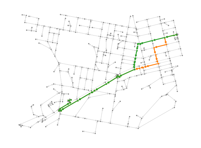
With a graph representation of the road network, we can find a route between any two nodes (if connected) with standard algorithms. The examples above and below uses Dijkstra’s algorithm to find shortest path based on edge weights that reflect our routing preferences. The orange route is “fewest hops” (count of road segments) and the green route is “shortest distance”. Geometric length of road segments is calculated in a post-processing pass over the ingested polyline data, and assigned as a weight to each edge.
Optimisation and scaling
My first spikes were hideously inefficient, but once the method was established, there was a lot of room for improvement. I addressed three major performance bottlenecks as I scaled from processing 50k undirected road segments in 50 minutes, to 1.1M directed road segments in 30 seconds. These figures represent a 2017 Macbook Pro, or free Colab instance, being roughly similar.
| Improving stage timings | 50k segments | 1.1M segments |
| Coincident segment endpoints | ||
| For loop accumulating unique ids with distance test | 50 mins | |
| numpy array calculation argwhere distance < e and numpig | 6 mins | |
| scipy.spatial.KDTree.query_pairs | 2 mins | |
| Shared node mapping | ||
| List comprehension elementwise map | Broke Colab | |
| numpy materialised mapping | < 2 mins | |
| Directed edges (previously undirected) | ||
| For loop accumulating correctly directed edges case-wise and discarding topological duplicates | > 12 hrs | |
| numpy vectorisation of loop conditional logic | 30 sec |
An additional ~30s is required to post-process geometric length of segments as an attribute per edge, and I imagine similar for other derived edge attributes. For instance, we might get finer grained average cycling speed per segment, or traffic risk factors, etc.
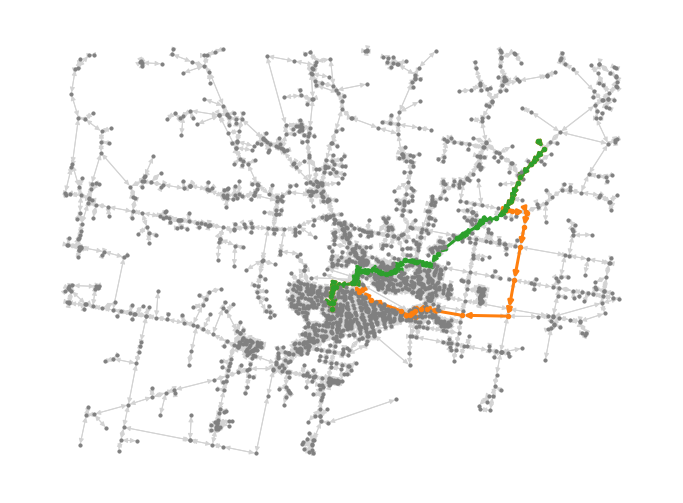
For calculating routes, (i.e., at inference time) it takes about 1-4s to find a shortest path, depending on the length of the route (using pure Python networkx). We can now find routes of over 950km length, from Mildura in the state’s north-west to Mallacoota in the east.

More latitude for navigation
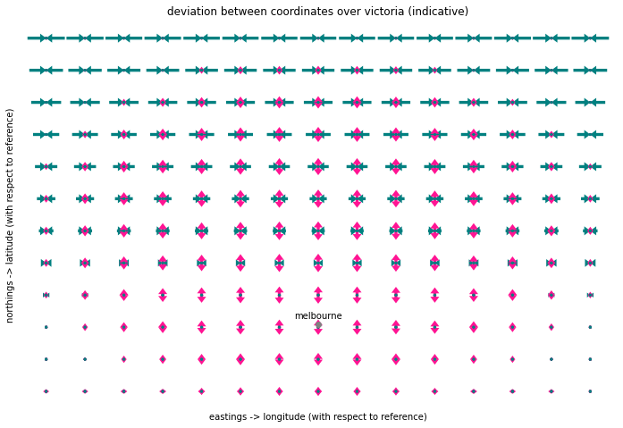
We would like to be able to find the start and end nodes of a route from latitude and longitude. However, as the nodes in our routing graph are located by VicGrid grid coordinates (eastings and northings), we first need to “wrap” this planar grid around the roughly spherical Earth. While geometrically complex (see below), it’s easy to do this transformation back and forth between coordinate systems with pyproj
Turn-by-turn navigation directions
With the start and end nodes located from latitude and longitude, a route can be calculated as above. Then, turn-by-turn directions can then be derived by considering the geometry of the road network at each intermediate node on the route, and what instructions might be required by users, for instance:
- Determine the compass direction of travel along a road segment to initiate travel in the correct direction,
- Calculate the angle between entry and exit directions at intersections to provide turn directions as left, right, straight, etc,
- Use the geometric length of road segments to provide distance guidance,
- Consolidate to a minimum set of directions by identifying where explicit guidance is not required (e.g., continuing straight on the same road), and
- Render the instructions into an easily (?) human-consumable form, with natural language descriptions of appropriate precision.
['travel south west on Holly Court',
 'continue for 190m on Holly Court',
 'turn right into Marigold Crescent',
 'continue for 360m on Marigold Crescent',
 'go straight into Gowanbrae Drive',
 'continue for 420m on Gowanbrae Drive',
 'turn left into Gowanbrae Drive',
 'continue for 150m on Gowanbrae Drive',
 'turn left into Lanark Way',
 'continue for 170m on Lanark Way']
This constitutes a rather neat first approximation to to commercial turn-by-turn directions, but I suspect it suffers in many edge cases, like roundabouts and slip lanes.
Next steps
With a drive-by look at the key elements, the road ahead to future “my way” hand-rolled navigation is clearer. An essential next step would be an interactive map interface. However, making this prototype roadworthy also likely needs more data wrangling under the hood (e.g., for cycling-specific data), a review of where to leverage existing open services, and polishing edge cases to a mirror finish.